
Trapped-ion system
05 October 2015
 \[\newcommand{\bra}[1]{\langle#1\rvert}
\newcommand{\ket}[1]{\lvert#1\rangle}
\newcommand{\braket}[2]{\langle #1| #2\rangle}
\newcommand{\braket}[3]{\langle#1\lvert#2\rvert#3\rangle}
\newcommand{\Yb}{^171\mathrm{Yb}^+}\]
\[\newcommand{\bra}[1]{\langle#1\rvert}
\newcommand{\ket}[1]{\lvert#1\rangle}
\newcommand{\braket}[2]{\langle #1| #2\rangle}
\newcommand{\braket}[3]{\langle#1\lvert#2\rvert#3\rangle}
\newcommand{\Yb}{^171\mathrm{Yb}^+}\]
A trapped-ion system uses ion traps to cool down and trap ions while the ions’ internal and motional quantum state are coherently manipulated by microwave or laser beams. Generally an ion trap is a manual designed combination of electric or magnetic fields that captures and confines ions in a free space region inside a vacuum system. Other than trapped ion quantum computers, ion traps have a number of important applications including mass spectrometery, precise measurement, and even world’s most accurate atomic clocks @Rosenband08. Two common types of ion traps are the Penning trap and the Paul trap (quadrupole ion trap). When using ion traps for scientific studies of quantum state manipulation, the Paul trap is most often used @Paul90.
In a trapped ion quantum computer, qubits are stored in long-lived stable electronic states of each ion. A universal set of gates is obtained by manipulating each ion’s internal states and collective quantized motional states of ion chains. Multi-ions’ entanglement can be prepared through the Coulomb force interactions and can be measured and transimitted with high fidelity. Quantum projection measurement is done by collecting quantized fluorescence photons from laser-induced emissions. The ultra-high vaccum (< $10^{-11}$ torr) and well designed harmonic trapping potential make trapped ions perfect pure quantum systems. Effective isolation from the outside environment noise and a rich set of operations make them constitute one of the most promising systems to implement scalable quantum computation and simulation.
In this chapter, I first introduce our 4-rod trap, which is the main platform I’m working on. Then there is some necessary theory preparations for trapped ion dynamics. In the last section we mainly describe how to realize our trapped-ion system.
4-rod trap
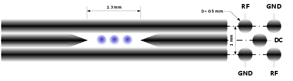
The 4-rod trap is one kind of Paul linear trap ↩. It uses 4 electrodes to form a rotating radio frequency field. The potential of the field can be described as a parabolic pseudo-potential on $x,y$ plane, centered at origin point, which makes the ions elastically bound to $z$ axis. And in the $z$ direction, 2 electrodes are used to generate a static coulomb potential, in which ions are arranged into a string. The total potential generated by these electrodes can be written as @Leibfried03
\[\begin{aligned} \Phi(x,y,z,t) & = U\frac{1}{2}(\alpha x^{2}+\beta y^{2}+\gamma z^{2})\\ &+\tilde{U}\cos(\omega_ {\mathrm{rf}}t)\frac{1}{2}(\alpha'x^{2}+\beta'y^{2}+\gamma'z^{2})\nonumber\end{aligned}\]where
\[\begin{aligned} -(\alpha+\beta) &= \gamma<0,\nonumber\\ \alpha'+\beta' &= \gamma'=0.\nonumber\end{aligned}\]The classical equations of motion of a ion with mass $m$ and charge $Z\lvert e\rvert$ in this potential can be decoupled in the spatial coordinates. The equation of motion in the $x$ direction can be written as a Mathieu differential equation
\[\begin{aligned} \frac{d^{2}x}{d\xi^{2}}+[a_ {x}-2q_ {x}\cos(2\xi)]x & = 0\end{aligned}\]where
\[\begin{aligned} \xi &= \frac{\omega_ {\mathrm{rf}}t}{2},\nonumber\\ a_ {x} &= \frac{4Z|e|U\alpha}{m\omega_ {\mathrm{rf}}^{2}},\nonumber\\ q_ {x} &= \frac{2Z|e|\tilde{U}\alpha'}{m\omega_ {\mathrm{rf}}^{2}}\nonumber.\end{aligned}\]The lowest-order approximation stable solution under the necessary condition $(\lvert a_ {x}\rvert,q_ {x}^{2})\ll1$ will be
\[\begin{aligned} x(t) & \approx 2AC_ {0}\cos(\beta_ {x}\frac{\omega_ {\mathrm{rf}}}{2}t)[1-\frac{q_ {x}}{2}\cos(\omega_ {\mathrm{rf}}t)]\\ \beta_ {x} & \approx \sqrt{a_ {x}+q_ {x}^{2}/2}\nonumber\end{aligned}\]The motion solution consists of secular harmonic oscillations at frequency $\omega_ {m}=\beta_ {x}\omega_ {\mathrm{rf}}/2\ll\omega_ {\mathrm{rf}}$ and a fast, small oscillations called ’micromotion’, which has the same frequency as RF field. If micromotion is neglected, the secular motion can be approximated by that of a harmonic oscillator with frequency $\omega_ {m}$. Later we will use this to obtain a quantum mechnical picture of trapped ion dynamics.

4-rod trap and vaccum chamber used in CQI.
Sometimes the ions’ default balanced position are shifted from the $z$ axis of the trap because of unsymmetric static electric field, usually caused by imperfect machining or assembling. At this time the micromotion of ions will become stronger. In order to prevent such effect, 2 extra cylindrical tungsten steel electrodes are added outside the trap to compensate the background electric field ↩. A $2$ ns resolution FPGA-based Time to Digit Converter(TDC) is built to measure the time correlation of ion’s micromotion frequency and its florescence rate along certain direction. We use this time correlation pattern as a directional indicator to adjust voltages that applied on these micromotion compensation electrodes. After we design the trap holder and whole assembling procedure with Autodesk Inventor, we use a simulation software called ’CPO3D’ is to simulate and verify all these electric fields.
We preprocess all 8 electrodes with electro chemical polishing for several minutes to remove rust and get a better cylinder shape. The heads of two DC electrodes in $z$ direction are then grinded to cones with sand papers. DC electrodes and RF electrodes are mounted with a pair of 5 holes ceramic tubes which are cutted and drilled by laser maching. However, the machining quality is always a limitation of making a stable trap even with a perfect design. As an example of efforts to overcome this kind of limitation, we make a lot of ceramic tubes and only choose the best matched pair for the real use. We take pictures of all tubes’ faces ↩ and then analyse them with a image processing program written in Mathematica. The same program has also been used to recognize and fit gaussian border of each ion within real-time ions crystal images.

find the best match of ceramic tubes pair.
Around the trap, 4 atomic ovens each filled with natural Yb, Yb 171, natural Ba and Ba 137 are mounted as atom sources. When a DC current of typically $2$A is applied to the stainless steel tube, the filling is heated up, then a beam of several thousand atoms is emitted from the oven to the trap ↩.
The strong RF field is provied by a homemade high quality amplifier working at around $12$ MHz, called ’helical resonator’ @Siverns11, which has a pretty high amplification (> 200) and a narrow bandwidth at the same time. The effective cavity length of helical resonator decides its resonance frequency and transimission ratio. A shielding box filled with styrofoam peanuts is built to protect helical resonantor from lab temperature flucatuation.

trapped ions. distance between two adjacent ions in first image is around $10$ $\mu$m.
All the vaccum components are cleaned ultrasonically several times in alternate baths of ethanol and acetone before final assembling. They are then ari-baked with a big high temperature oven before assembling to acquire a chromium oxide coating. This coating is able to prevent the material of vacuum components from absorbing gases in the air, thus decreasing the amount of out gassing. We use a 4 levels vacuum pump system (mechanical pump, turbo pump, big ion pump, small ion pump and Ti sublimation pump) to prepare a ultra high vacuum environment (see in Fig. ↩). When the vaccum is below $10^{-8}$ torr, $H_ 2O$ is the mainly remained molecule. So the big oven is again used for vacuum-baking. It heats the vacuum system to around $200\ ^\circ\mathrm{C}$ for about one week to speed up the outgassing process and completely vaporize the water layer. When the baking was finished, the bakeable valve was sealed before the temperature starts to decrease, to cut off the inner vaccum system from the outer pumps. A RGA leakage detector and an ionization vacuum meter are also used to check and verify vacuum during the whole vaccum-preparation stage. Finally, when the system is at room temperature, the Ti sublimation pump is turned on to take out the remaining hydrogen, which is the dominant ingredient in UHV environment. With this whole procedure we can archive a ultra high vaccum near to $10^{-12}$ torr, under which the collision frequency will be as low as $21$ hours. This makes our ions extremely stable: ion seldomly disappear during experiments and can survive over nights even without laser cooling.

vacuum pump system and big oven.
Trapped ion dynamics
Internal electronic level structure of the ion
For a lot of experiments, we use ion’s clock transition as a qubit. The internal electronic structure of the ion will be approximated by a 2-level system with levels $\ket g$ and $\ket e$ of energy difference $\hbar\omega_ 0=\hbar(\omega_ {e}-\omega_ {g})$. The corresponding two-level Hamiltonian is
\[\begin{aligned} \hat{H}^{(e)} & = \hbar(\omega_ {g}\ket g\bra g+\omega_ {e}\ket e\bra e)\\ & = \hbar\frac{\omega_ {e}+\omega_ {g}}{2}(\ket g\bra g+\ket e\bra e)\\ & + \hbar\frac{\omega}{2}(\ket e\bra e-\ket g\bra g)\\ & = \hbar\frac{\omega_ {e}+\omega_ {g}}{2}\bf I + \hbar\frac{\omega_ 0}{2}\sigma_ {z}\end{aligned}\]Since we will consider the evolution in the interaction picutre, the constant part can be safely eliminated and only the $\sigma_ {z}$ part remains. This elimination can be easily extend to a N-level system
\[\begin{aligned} \hat{H}^{(e)} & = \hbar\sum_ {i=1}^{N}\omega_ {i}\ket i\bra i\rightarrow\hbar\sum_ {i=1}^{N}(\omega_ {i}-\omega_ {1})\ket i\bra i\end{aligned}\]Quantum-mechanical equations of motion
For the quantum-mechanical treatment of the motion, replacing the coordinate $x$ by the respective operator $\hat{x}$, we can write the time-dependent potential $V(t)$ as
\[V(t)=\frac{m}{2}W(t)\hat{x}^{2}\]where
\[W(t)=\frac{\omega_ {\mathrm{rf}}^{2}}{4}(a_ {x}+2q_ {x}\cos(\omega_ {\mathrm{rf}}t))\]can be thought of as a time-varying spring constant that will play a role similar to $\omega^{2}$ in the static potential harmonic oscillator. With these definitions, the Hamiltonian of the motion $H^{(m)}$ takes a form very similar to the familiar Hamiltonian of a static potential harmonic oscillator
\[\hat{H}^{(m)}=\frac{\hat{p}^{2}}{2m}+\frac{m}{2}W(t)\hat{x}^{2}=\omega_ {m}a^{\dagger}a\]Typically the trap frequency $\omega_ m$ = ….
Interaction hamiltonian
We can interact with ion by applying an external wave field from either microwave horn or laser beam. For dipole allowed transitions the field will be treated in the familiar dipole approximation, while for dipole forbidden transitions only the quadrupole component of the field is considered. For Raman transitions, the near-resonant intermediate level will be adiabatically eliminated, making these transitions formally equivalent to the other transition types.
Electric dipole allowed transitions, electric quadrupole allowed transitions, and stimulated Raman transitions can be described in a unified framework that associates a certain on-resonance Rabi frequency $\Omega$, effective light frequency $\nu$, and effective wave vector $\vec{k}$ with each of these transition types. The effective light frequencies and wave vectors are identical to the frequency and wave vector of the coupling light field for dipole and quadru pole transitions, but equal to the frequency difference $\nu=\nu_ {1}-\nu_ {2}$ and wave vector difference $\vec{k}=\vec{k}_ {1}-\vec{k} _ {2}$ of the two light fields driving the stimulated Raman transitions. For running wave light fields all three transition types can be described by a coupling Hamiltonian of the form
\[\begin{aligned} \hat{H}^{(i)}&=\hbar\Omega(\hat{\sigma}_ ++\hat{\sigma}_ -)\cos(k\hat{x}-\nu t+\phi)\\ &=\frac{\hbar}{2}\Omega(\hat{\sigma}_ ++\hat{\sigma}_ -)e^{\imath(\eta(\hat{a}+\hat{a}^\dagger)-\nu t+\phi)}+h.c. \end{aligned}\]where the Lamb-Dicke parameter $\eta=kx_ {0}$, $x_ {0}=\sqrt{\hbar/(2m\omega_ m)}$ is the extension along the $x$ axis of the ground-state wave function.
Now we have the total Hamiltonian in Schoedinger picture
\[\hat{H}=\hat{H}^{(e)}+\hat{H}^{(m)}+\hat{H}^{(i)}\]If we label spin ground state as $\ket{\downarrow}$, excited state as $\ket{\uparrow}$, motional state as $\ket{n}$, then for transition $\ket{\downarrow,n}\leftrightarrow\ket{\uparrow,m}$, we can choose the interaction picture with respect to external field’s frequency. The base Hamiltonian
\[\hat{H}_ 0=\hat{H}^{(e)}+\hat{H}^{(m)}+\frac{\hbar\delta}{2}\sigma_ z\]where the detuning from resonance $\delta=\nu-\omega_ 0-(m-n)\omega_ m$, and the coupling term
\[\begin{aligned} \braket{\uparrow,m}{\hat{H}_ I}{\downarrow,n}&=\braket{\uparrow,m}{e^{\imath\hat{H}_ 0 t/\hbar}(\hat{H}-\hat{H}_ 0)e^{-\imath\hat{H}_ 0 t/\hbar}}{\downarrow,n}\\ &=e^{\imath(1/2(\omega_ 0+\delta)+m\omega_ m+1/2(\omega_ 0+\delta)-n\omega_ m) t}\braket{\uparrow,m}{\hat{H}^{(i)}-\frac{\hbar\delta}{2}\sigma_ z}{\downarrow,n}\\ &=e^{\imath\nu t}\braket{\uparrow,m}{\frac{\hbar}{2}\Omega(\hat{\sigma}_ ++\hat{\sigma}_ -)e^{\imath(\eta(\hat{a}+\hat{a}^\dagger)-\nu t+\phi)}+h.c.}{\downarrow,n}\\ &=\frac{\hbar\Omega}2\braket{ m}{e^{\imath(\eta(\hat{a}+\hat{a}^\dagger)+\phi)}+e^{\imath(-\eta(\hat{a}+\hat{a}^\dagger)+2\nu t-\phi)}}{\downarrow,n} \end{aligned}\]Apply rotating-wave approximation
\[\begin{aligned} \braket{\uparrow,m}{\hat{H}_ I}{\downarrow,n} &\approx\frac{\hbar\Omega}{2}e^{\imath\phi}\braket{m}{e^{\imath\eta a^\dagger+\imath\eta a}}{n}\\ &=\frac{\hbar\Omega}2 e^{-\frac{\eta^2}2+i\phi} \braket{m}{e^{i\eta a^\dagger} e^{i\eta a}}{n}\\ &=\frac{\hbar\Omega}2 e^{-\frac{\eta^2}2+i\phi} (\sum_ {j=0}^\infty\frac{(\imath\eta)^j}{j!}(a^\dagger)^j\bra{m})\cdot(\sum_ {j=0}^\infty\frac{(\imath\eta)^j}{j!}a^j\ket{n})\\ &=\frac{\hbar\Omega}2 e^{-\frac{\eta^2}2+i\phi} (\sum_ {j=0}^m\frac{(\imath\eta)^j}{j!}\sqrt{\frac{m!}{(m-j)!}}\bra{m-j})\cdot(\sum_ {j=0}^n\frac{(\imath\eta)^j}{j!}\sqrt{\frac{n!}{(n-j)!}}\ket{n-j})\\ &=\frac{\hbar\Omega}2 e^{-\frac{\eta^2}2+i\phi} (\sum_ {k=0}^m\frac{(\imath\eta)^{m-k}}{(m-k)!}\sqrt{\frac{m!}{k!}}\bra{ k})\cdot(\sum_ {k=0}^n\frac{(\imath\eta)^{n-k}}{(n-k)!}\sqrt{\frac{n!}{k!}}\ket{k})\\ &=\frac{\hbar\Omega}2 e^{-\frac{\eta^2}2+i\phi} \sum_ {k=0}^{n_ <}\frac{(\imath\eta)^{m+n-2k}\sqrt{m!n!}}{(m-k)!(n-k)!k!}\\ &=\frac{\hbar\Omega}2 e^{-\frac{\eta^2}2+i\phi}(\imath\eta)^{n_ >-n_ <}\sqrt{\frac{n_ < !}{n_ >!}} \sum_ {k=0}^{n_ <}\frac{(\imath\eta)^{2(n_ <-k)}}{(n_ <-k)!}\frac{n_ >!}{(n_ >-k)!k!}\\ &=\frac{\hbar\Omega}2 e^{-\frac{\eta^2}2+i\phi}(\imath\eta)^{n_ >-n_ <}\sqrt{\frac{n_ < !}{n_ >!}} \sum_ {k=0}^{n_ <}(-1)^{n_ <-k}\binom{n_ >}{k}\frac{(\eta^2)^{n_ <-k}}{(n_ <-k)!}\\ &=\frac{\hbar\Omega}2 e^{-\frac{\eta^2}2+i\phi}(\imath\eta)^{|m-n|}\sqrt{\frac{n_ < !}{n_ >!}} \sum_ {j=0}^{n_ <}(-1)^j\binom{n_ <+|m-n|}{n_ <-j}\frac{(\eta^2)^j}{j!}\\ &=\frac{\hbar\Omega}2 e^{-\frac{\eta^2}2+i\phi} (i\eta)^{|m-n|}\sqrt{\frac{n_ < !}{n_ >!}}L_ {n<}^{|m-n|}(\eta^2) \end{aligned}\]where Laguerre polynomial
\[L_ n^\alpha(x)=\sum_ {j=0}^n(-1)^j\binom{n+\alpha}{n-j}\frac{x^j}{j!}=\binom{n+\alpha}{n}-\binom{n+\alpha}{n-1}x+\cdots\]So
\[\braket{\uparrow,m}{\hat{H}_ I}{\downarrow,n} \approx \frac{\hbar\Omega}2 e^{-\frac{\eta^2}2+i\phi} (i\eta)^{|m-n|}\sqrt{\frac{n_ < !}{n_ >!}}\left(\binom{n_ >}{n_ <}-\binom{n_ >}{n_ <-1}\eta^2\right)\]Specially, for carrier transition $ |\downarrow,n\rangle\rightarrow |\uparrow,n\rangle$
\[\hat{H}_ I\approx\frac{\hbar\Omega}2 e^{-\frac{\eta^2}2}\left( \sigma_ +e^{i\phi}+h.c \right) -\frac{\hbar\delta}2\sigma_ z\]For blue sideband $ |\downarrow,n-1\rangle\rightarrow |\uparrow,n\rangle$, and red sideband $ |\downarrow,n\rangle\rightarrow |\uparrow,n-1\rangle$
\[\hat{H}_ I \approx\frac{\sqrt n\hbar\Omega}2 \eta e^{-\frac{\eta^2}2}\left[ \sigma_ + e^{i(\phi+\frac{\pi}{2})} +h.c \right] -\frac{\hbar\delta}2\sigma_ z\]The ion system
Currently all our experiments are using the ion. We use the optical transition $^{2}S_ {1/2}\leftrightarrow^{2}P_ {1/2}$ as a main cycle for Doppler cooling, state initialization and detection. The hyperfine level $\ket{F=0,m=0}$ and Zeeman splitting levels $\ket{F=1,m=0,\pm1}$ are used together as a 4-level system.

relevant levels of the $\Yb$ @Chew08
Basic procedures
Once the Yb 171 oven is heated up by applying certain current, the Yb 171 metal inside will melt and gasify, then a beam of Yb 171 atoms will shoot towards the trap. A $\sim500\mu$W $398.9108$ nm beam provided by Toptica diode laser and a $\sim5$mW $369.5263$ nm beam provided by Toptica SHG laser will hit some Yb 171 neutral atoms and ionize them to ions. Both beams are focused to $\sim50\mu$m waist at the center of trap. The ion will then be confined near to the center of trap. At this time, the ion is still very hot and not stable in the trap. Another pair of beams are used to Doppler cool it down. One of them is a $\sim50\mu$W $369.5263$ nm beam, slightly red-detuned from the optical transition $^{2}S_ {1/2}\leftrightarrow^{2}P_ {1/2}$. The ion on $^{2}S_ {1/2}$ can absorb one laser photon and go up to $^{2}P_ {1/2}$, the life time of $^{2}P_ {1/2}$ is only $8.7$ns, then it spontaneously emits a photon to every direction with uniformly probability distribution.

load and trap with lasers.
Since the ion keeps oscillating in the trap, ion’s momentum along laser’s direction will be efficiently cancelled after hundreds of thousands cycles, within $1$ms. This beam has a $14.74$ GHz sideband provided by a LabBrick driven Electro-Optic Modulator(EOM), to cover all possible transitions between hyperfine levels. The second one is an auxiliary but important $\sim10$mW $935.1882$ nm beam. It’s used to repump $0.5\%$ leakage on metastable $^{2}D_ {3/2}$ back to the main cycle, thus completes a stable Doppler cooling scheme. This beam also has a $3.1$ GHz sideband. Sometimes the ion falls into the $^{2}F_ {7/2}$ state, possibly caused by collisions with residual background gas. A $\sim1$mW laser beam near $638.6101\sim638.6151$ nm depopulates the $^{2}F_ {7/2}$ level and returns the ion to the four-level Doppler cooling scheme. This whole ion trapping procedure is usually called ’load’ ion ↩.
Another $369.5263$ nm optical pumping beam is used to intialize ion to state $\ket{F=0,m=0}$, labelled as state $\ket 1$ in our 4-level system. Unlike Doppler cooling beam, the optical pumping beam is modulated with a $2.105$ GHz EOM. Its sideband doesn’t cover transitions from $\ket{F=0,m=0}$, which means $\ket{F=0,m=0}$ will never be excited, but other states can go down to $\ket{F=0,m=0}$ by spontaneously emission. So after a bunch of cycles ($\sim5\mu$s), the ion will be on state $\ket{F=0,m=0}$ with high fidelity (> 99.5%).
All these laser beams are finally applied to trap center through lenses and small view ports on the vaccum chamber. Each lens is mounted to a three dimensional transition stage, which provides a firm support as well as a precise control of the optical system. In alignment for addressing ions, usually we use shadows or CCD camera images of rods and needles to determine the geometry center of our trap.

370nm laser optical paths.
A two stage optical observation system designed with the OSLO software is set up to collect florescence coming from the ion ↩. A microscopic objective lens with a short focal length and a large numerical aperture is used as the first stage of detection, to maximize the solid angle (0.77%) of the detection lens to the ion. A group of magnifying lenses at the second stage casts the image to the sensitive surface of optical detection devices. We put a CCD camera at one end of the second stage to observe ions and help align optical beams and a PMT at another end to count emitted photons. Observation with CCD or PMT is switchable by a flipping mirror. Two $370$ nm narrow-band filters are inserted into the optic tubes to filter out background noise introduced by photons of other wavelength. The population on state $\ket 1$ can be measured by a $369.5263$ nm detection beam only resonant to $^{2}S_ {1/2,}F=1\leftrightarrow^{2}P_ {1/2},F=0$ transition. If the emitted photon counting rate is higher than detection threshold $\sim1/300\mu$s, the population is $0$, otherwise $1$.

detection system with CCD and PMT.
We put magnets or Hermholtz magnetic coils on top of vacuum chamber to provide a quantization axis and to maintain certain Zeeman splittings. Zeeman splitting levels $\ket{F=1,m=-1,0,1}$ are labelled as state $\ket 2,\ket 3,\ket 4$ in our 4-level system. The energy gap between state $\ket 1$ and state $\ket 2$, is $\sim12.64$ GHz. The energy gap between $\ket 2,\ket 3$ and $\ket 3,\ket 4$ are $\sim1.4$B MHz/gauss, where B is the static magnetic field strength at ion’s position, typically $\sim10$ gauss with coil current $\sim3$A.
For the quantum operations with microwaves ↩, the main device we control is a $1$ GHz sampling rate PCI-board Arbitrary Waveform Generator(AWG). It’s used to generate arbitrary waveforms from $186\sim214$ MHz. The ouput of AWG is then mixed with a $\sim12.44$ GHz microwave provided by an Agilent microwave source. Both them are externally referenced by a $10$ MHz Rb atomic clock. After amplification with fan and water cooled 2-level amplifer system, microwave finally applies to the trap through a horn antenna. The microwave forms a standwave inside the chamber. We can adjust polarization or strength by moving or rotating the microwave horn. With some sort of optimization, currently the Rabi flopping $\pi$ times between $\ket 1$ and $\ket 2,\ket 3,\ket 4$ are $\sim1.5\mu$s, $4\mu$s, $1.5\mu$s, with fidelity > 98.5%.

quantum operations with microwave.
Let’s summarize the basic procedures to use this ion system:
-
Doppler Cooling. Cool down the ion.
-
Optical Pumping. Initialize to state $\ket 1$.
-
Microwave Manipulating. Rotate state coherently.
-
Florescence Detecting. Measure population of state $\ket 1$.
Laser frequency stablization
Efficient quantum operations on ions require that the $369.5263$ nm and $935.1882$ nm lasers are stable in frequency, especially the $369.5263$ nm laser, to well within the linewidths of the relevant transitions in the experiment. Normally diode lasers are very sensitive to temperature and current and will have huge fluctuation without further stablization. So we lock the $739.0526$ nm laser (after SHG becomes a $369.5263$nm laser) to a Fabry-Pérot(F-P) cavity using Pound–Drever–Hall(PDH) method to compensate fast fluctuation. The F-P cavity’s length is then externally locked to an absolute frequency reference provided by an Iodine vapor cell system, to compensate long term drift, mainly caused by temperature. A $\sim 13$ GHz fiber EOM is used to shift laser frequency to Iodine’s spectrum. This lock system ↩ works well, lasts as long as several days and results in a high precision $<1$ MHz. Lock point can also be easily controlled by changing fiber EOM’s driving frequency with a LabVIEW program running on the main control computer.

cavity and Iodine laser lock.
There are two kinds of important electronic devices used in a lock system. The first one is the PID. PID is the abbreviation of Proportion, Integration and Differentiation. A PID accepts an error signal input from the deviating device, does some calculation and then outputs a feedback signal to the regulating device. In this manner it is suitable for real-time automatic control, lock or synchronization. As its name shows, the calculation unit of a PID consists of 3 components and outputs the weighted summation of them as the final feedback signal. In principal we can make an automatic feedback loop for arbitrary system by setting appropriate coefficients of 3 components. Another important kind of device is the Lock-In amplifier, which is very useful to pick up weak signals from a noisy background. It takes advantage of the orthonormality of trigonometric functions:
\[\int_ {-\pi}^{\pi} \cos(mx)\, \cos(nx)\, dx = \pi \delta_ {mn}, \quad m, n \ge 1.\]If we multiply a noisy signal with a reference signal and do integration, then all signals except the one with the same frequency as the reference signal vanish. The Lock-In amplifier is just the device that can simulate this mathematical process, which has a mixer to do multiplication, a low pass fiter to throw away high frequency components, and an integrating circuit to do the final integration. The directly measured deviation signal is always very noisy because of power fluctuation and looses directional information which is essential for a feedback loop. So in a lock system, we usually apply some low frequency modulation on the source signal, then use a Lock-In amplifier to pick up the carried amplitude envelope of that low frequency, which can be seen as the directional derivative signal with respect to frequency.
In our cavity lock system, the PDH module inside controller box of 740nm Toptica diode laser puts voltage modulation with frequency $\omega_ m$ on the diffraction grating piezo of external cavity diode laser. The output laser light of frequency $\omega$ is then phase-modulated by $\beta\sin(\omega_ m t)$, which can be represented by its electric field with one carrier and two sidebands
\[\begin{aligned} E &= E_ 0 e^{i( \omega t+\beta\sin(\omega_ \mathrm{m} t))} \\ &\approx E_ 0 e^{i\omega t} [1+i \beta \sin(\omega_ \mathrm{m} t)] \\ &= E_ 0 e^{i \omega t}\left[1+\frac{\beta}{2}e^{i\omega_ \mathrm{m} t}-\frac{\beta}{2}e^{-i \omega_ \mathrm{m} t}\right].\end{aligned}\]Phase modulation is also widely implemented by EOMs or Acoustic-Optic Modulator(AOM)s in our laser setup to enrich frequency components. The reflection power signal about laser frequency for our F-P two mirror cavity is a single peak function with a similar shape to a sharp normal distribution function. The PDH module takes this reflection signal from the photodetector and extracts the directional derivative signal with a circuit consists of a phase shifter, a mixer and a low pass filter, which has a similar function to a Lock-In amplifier. For certain cavity length, the sharp center slope of derivative signal indicates how far laser’s frequency is deviated from cavity’s resonance laser frequency. The signal’s sign is always the same as the sign of target frequency minus current frequency, and is suitable as an error signal for the PID to compensate laser’s frequency. The PID’s DC output is then added to the piezo of external cavity diode laser, thus keeps output laser’s frequency synchronized with, i.e., locked to cavity’s resonance laser frequency. More formal and mathematical description of this PDH method can be found in PDH’s original paper @PDH83.
With the one body high finesse confocal cavity designed by ourself and made of hard indium steel, the cavity lock system is really stable, which can even tolerate huge mechanical hit while keep the lock. The ultra low heat expansion rate of indium steel material also makes our cavity’s length insensitive to lab temperature. However, to lock the $739.0526$ nm laser in $1$ MHz($\approx 1.8$ fm) region, for a $15$ cm cavity, the desired cavity length’s fluctuation should be within \(\frac{2L}{\lambda}\Delta\lambda=\frac{2L\lambda}{c}\Delta f\approx0.74\mathrm{nm}.\) To fulfill this requirement, one way is to put our cavity into a highly isolated environment, such as vaccum or cryostat, which is also helpful to cavity’s finesse. Another simpler way is to use some absolute frequency reference to lock cavity’s length, like a Rb-stabilized cavity. This way depends on the existence of absolute reference near your target frequency. Fortunately, Iodine molecule has a absorbing peak at $13531.2773\ \mathrm{cm}^{-1}$ @Olmschenk07, which is corresponding to wavelength $739.028532$ nm and is close to our target wavelength. Iodine is solid under normal condition. It’s put into a vaccum vapor with a cold finger. The vapor is surrounded with heating tapes to keep it in around $\sim 300\ ^{\circ}\mathrm{C}$ high temperature, under which Iodine gasify and fill into whole vapor. The directly measured absorbing peak of hot Iodine molecules is shifted by Doppler effect because of their quick motion. So we use two opposite laser beams to get the saturated Doppler-free signal. One of the beam is also phase modulated with a $15$ KHz signal for the usage of Lock-In amplifier, through a $80$ MHz center frequency AOM. The error signal outputs from the Lock-In amplifier indicates laser frequency deviation from Iodine’s absorbing peak. This error signal is feeded into another PID and feedbacks to the $\pm 75$ V high voltage board which finally stabilizes, i.e., locks the length of cavity. By changing input frequency of the fiber EOM which bridges the lock target frequency with Iodine’s absorbing peak, we can precisely control our laser’s frequency relative to some absolute reference.
The $935.1882$ nm is directly locked to a HighFinesse wavelength meter with precision $\sim10$MHz. A custom program written in Visual Basic is used to auto-calibrated the wavelength meter every $10$ seconds to compensate wavelength meter’s long term drift, using the already stablized $739.0526$ nm laser’s wavelength as a reference.
Control units
Once we have the ability to change all necessary properties of our traps and lasers, the next step is to build some accessible and reliable electronic units that have integrated control over all these apparatus. The voltage of each micromotion compensation electrode as well as axial confinement electrode in our trap can be individually controlled through an ISEG high voltage module. A custom control program written in LabVIEW is used to change some of these electrodes’ voltages simultaneously with arbitrary ratio. All EOMs for adding frequency sidebands or changing lock points are controlled by LabBrick signal generators, which are connected to control computers through USB cables and there are nice software interfaces that let us control them with mouses and keyboards. AOMs are mainly served as optical switches to control the duration of laser beams with nanosecond to microsecond level precisions. We use signal generators as drivers to control the modulation frequencies and strengthes of them. The output states of these signal generators are then controlled by RF switches which can be quickly opened or closed in $< 5$ ns through TTL signals generated by a high performance TTL sequence generator as it shows in Fig. ↩. To maintain a stable time and phase relationship between operations, high frequency signal generators as well as TTL sequence generators are all finally referenced by a same $10$ MHz Rb atomic clock reference ring.

$24$ ports pulse sequencer. bottom is a RF switches box it controls.
We build our own 20 channels TTL sequence generator @Zjh12, from a general-purpose Altera Cyclone EP2C5T144C6 FPGA board, which is now upgraded to a 28 channels version with much higher instruction capacity from a Cyclone EP3C25 board. A $4$ channels $24$ ($32$ for upgraded version) bits gated counter is also programmed inside this pulse sequencer on the same board to ouput photon counts measured by PMT in real-time. To achieve high time resolution of output signals, the onboard PLL is used to divide input $50$ MHz clock frequency up to $500$ MHz. A $5$ First-In-First-Out(FIFO)s assembly-line parallel scheme is implemented to distribute the read-convert procedure of about $10$ ns into $5$ clock cycles to achieve a minimal segment duration of $2$ ns. The binary format of all instruction flows about time sequences or counters are carefully designed to be highly compact and easy to process and dispatch by FPGA circuits. With these hard optimizations, our pulse sequencer is able to manage $24$ ($32$ for upgraded version) independent ports, with a range of durations from $2$ ns to $4.2$ ms ($5497.5$ s for upgraded version) and a maximum of $2560$ ($7680$ for upgraded version) segments in length.
Chapter(DopplerCooling,
00000000 00000000 00000000)
Chapter(OpticalPumping,
11000000 00000000 00000000)
Chapter(Detection,
10100000 00000000 00001111,
10000000 00000000 00000000,
10000000 00000000 00010000)
Chapter(AWG,
10010000 00000000 00000000)
Chapter(Zero,
10000000 00000000 00000000)
DopplerCooling(1000)
OpticalPumping(5)
AWG(100)
Detection(300,1,1)
Zero(30)
The pulse sequences used in our experiments usually consists of many pulse segments, each pulse segment is a continuous period when all ports have constant states. The binary packet of each segment contains bits to describe its duration and each port’s state. Each duration is a special encoded timestamp with a unit of minimal time resolution, which represents the number of clock cycles for this packet. The state bits are just the literally represention of all ports’ boolean states. Every packet has the same fixed bit width. The start packet is unique and contains the number of repeations for this whole pulse sequence, as well as a start flag bit and an external trigger flag bit. This binary protocol is of high efficiency and friendly to FPGA circuits. A simple text-based language is also developed to add human readability and can be easily translated to its binary equivalent by computer programs. In the example sequence file in Fig. ↩, the “Chapter definitions” part associates chapter names with some boolean states of $24$ ports in our pulse sequencer. In the “Sequence body” part, we can use the chapter name to represent the associated boolean state. Each argument number inside parentheses represents the duration of each state in the unit of microsecond. The corresponding time sequence diagram for the first $4$ output channels A$0$ to A$3$ is showed in Fig. ↩. Note that the time scale has only relative meaning for better readability. channel A$0$ is connected to the RF switch which controls the AOM of Doppler cooling beam path. The RF switch is reverse used and its state is ON by default, when the pulse sequencer outputs 0 so that the TTL input of RF switch is low level. channel A$1$ controls optical pumping beam path and channel A$2$ controls detection beam path. The Detection segment has another two $1\ \mu$s sub-segments after the detection beam path opens for $300\ \mu$s. These 2 sub-segments have no output effects but internally they control the integrated gated counter to send TTL input counts data of the real detection segment back to the control computer. channel A$3$ connects to the external trigger input of our AWG board, thus controls the start time of microwaves.

time sequence diagram of sequence file in Fig. ↩.
From this simple example we notice that TTL signals are really good messengers which bridge the analog world with the digital world. In principle we can use TTL signals to control any finite state machines, which means any devices with finite and discrete possible operations. With this ability of precisely arranging the time order of all operations, the pulse sequencer actually serves as the center control unit of our trapped-ion system. The pulse sequencer, together with all these control units which can talk with computer as well as other devices, form the important bottom layer of our integrated control system.
Software architecture
From the point view of software engineering, all devices in the lab makes a complex heterogeneous system. Unlike computers, most devices doesn’t run an operating system. Many devices even doesn’t have a single chip on it. Also there are a bunch of different kinds of physical communication methods for different devices, from the simplest TTL trigger signal to the internet connection. Fortunately, on top of the abstract layer of control units, we only need to deal with machines which are able to talk with computers. As the pulse sequencer serves as the center control unit, naturally the software that talks with the pulse sequencer should also be in the center of our software architecture. In our system, this main control software is a graphical interface program written in LabVIEW as it shows in Fig. ↩. Its basic function is to communicate with the pulse sequencer through a $2\sim 4$ Mbps serial connection. We can load or edit sequence file on its left “Sequence” panel. The program can translate the text-based sequence language to binary bytes and send them to the pulse sequencer. If the sequence involves with gated counter channels which are usually used for collecting PMT counts, then the program can receive PMT counts data from the pulse sequencer and display average counts or states on the right “PMT” panel.

the main control program written in LabVIEW.
This basic input-output operation cycle is essential for all complex trapped-ion experiments. Usually one experiment is carried out repetitively with one parameter changing to obtain the relationship between the outcome and the parameter. The most common used two patterns are alignment sweeping and linear scanning. The “Sweep” button is used to start an alignment sweeping. In this case the software just repeatedly sends sequences and receives data. So we can adjust some external parameters such as optical alignments, and use this “trapped-ion oscilloscope” as a reference. In the case of linear scanning, instead of manually changing external parameters, we can tell the software which parameter we want to scan as well as the scanning range. During the scan, every parameter and its corresponding original data is recorded and organized into a table. After the scan, this table is converted to a flexible structured text-based format and is stored into our network file system in a uniform naming/path manner. The scanning parameter can be the duration of some segment in the sequence, or parameter of some other device which is integrated controlled by the sequencer software. Currently we integrate 2 most commonly used devices into the sequencer software. The first one is the LabBrick signal generator for the fiber EOM, which is used to control the lock frequency of our $370$ nm laser. Another one is the AWG board which can generate arbitrary waveforms for the implementation of complex hamiltonians. The AWG board is another main device in our system and is the key part to both microwave and Raman laser operations. The board’s driver library accept a number array and output the interpolation voltages with a fixed $1$ GHz sampling rate. In reality, the quantum gates or hamiltonians we implement can always be represented as a piecewise analytic function. So we define a CSV-based wave file format which has a segments structure and each segment has several standard parameters. In the example wave file Table ↩, the first line with a empty “Formula” field represents a standard cosine waveform a*cos(w*t+p), where a refers to Amplitude field $0.4$, w refers to $2\pi$ times the “Frequency” field $189.4681$ MHz and p refers to “Phase” field $0$. The second line has a similar explanation, except that g0 refers to “Gap” field in the first/0th line. This wave file is used for Ramsey measurement of state $\ket{2}$, we can scan the “Gap” parameter of the first line. The data we get should be a sine curve about this “Gap” and population of state $\ket{2}$, whose frequency is just the frequency gap between the Ramsey frequency of $\ket{2}$ and the “Frequency” field in the wave file. We can then use sine curve data fitting to calculate the correct Ramsey frequency. There are a lot of other functions and variables can be used in the formula field, thus makes this wave file format expressive enough for our quantum operations. The segment and parameter structure also makes it highly compatible with the linear scanning operation pattern.
| Frequency | Duration | Amplitude | Phase | Gap | Formula |
|---|---|---|---|---|---|
| 189.4681 | 1.156 | 0.4 | 0 | 1. | |
| 189.4681 | 1.156 | 0.4 | 0.5 | 1. | a*cos(w*(t-g0)+p) |
an example wave file for Ramsey measurement.
The main control program is released with a rich set of remote control interfaces so that it’s very easy to write some other software to share and make use of this main control resource. For example, we build a special control program for the condtional sequential measurement without breaking any existing code, by exchaning data with the main control program through a shared memory interface. Through its network interface, we can even run quantum operations and take data from another personal computer outside our lab. Note that this interface is for the experimental data layer instead of the user interface layer and is different from any remote desktop tricks. In this manner, the main control program effectively acts as a virtual device for other programs. All of these graphical interface programs form the second layer of our integrated control system.
Up to this graphical interface layer, we can already handle all the daily operations and do many experiments. However, for experiments with very complex logic, a text-based script language is desired to organize all complex operations. At first we use an embeded Lua engine to script our LabVIEW programs. It saves us a lot of time when we take data for the quantum contextuality and random number experiments. But it’s still not a perfect solution since we have to manually convert our quantum gates or hamiltonians into some form of program statements. I finally solve this problem by building a Mathematica-to-LabVIEW bridge. With this bridge, we develop an easy to use theory to experiment framework ↩, including numerical simulation, experimental sequence/wave generation, parameter calibration, data taking, data analysis and plotting, all of which are totally automatic once we write the initial theory definitions in Mathematica. Nowadays I also develop a Foreign Language Interface(FFI) for Mathematica, with which we can invoke native Dynamic Linked Libraries(DLL) and communicate with physical devices directly for efficiency critical reasons. Now this Mathematica-based automated control framework is the unified top layer of our integrated control system. A lot of fancy quantum computation and simulation experiments have been done with the help of this framework. I believe we are on the right way towards the ultimated software architecture of a quantum computer.

the diagram of IonTrap package written for Mathematica.